Digital Signal Processing Part 1: The Frequency Domain and the Fourier Transform
[dsp (Note: While I try to keep things as simple as possible, some basic knowledge of signals is assumed)
The Frequency Domain
When we look at signals, we tend to look at them from the perspective of the time domain (i.e. we look at how signals vary with time). In signal processing, we very frequently (heh) also look at signals in the frequency domain, where we can see how a signal is distributed across different frequency bands.
One core concept of signals is this: any signal can be represented as a sum of sinusoids. The general expression for a sinusoid at frequency $\omega$ rad/s (or frequency $f$ in Hz) is:
\[x(t) = a \sin(\omega t + \phi) = a \sin(2 \pi f t + \phi)\]Using the above expression, we can break down any signal into a series of sinusoids. This series is known as a Fourier series.
Here’s an example of a signal that is made up of two sine waves:
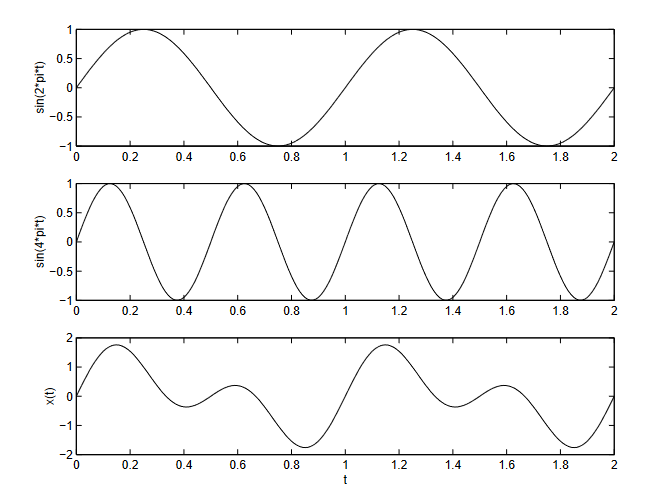
The top plot is the plot of $\sin (2 \pi t)$ and the middle plot is the plot of $\sin (4 \pi t)$. When we sum these two sinusoids, the result is the sinusoid in the bottom plot.
Here’s another more complex example. The red curve is a sum of sinusoids that approximates the blue curve, which is a square wave.
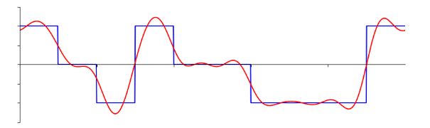
The more sinusoids we use, the better we can approximate the square wave.
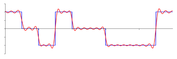
With an infinite number of sinusoids, we can perfectly approximate any signal.
Now let’s look at a sine wave, in both the time domain and frequency domain:
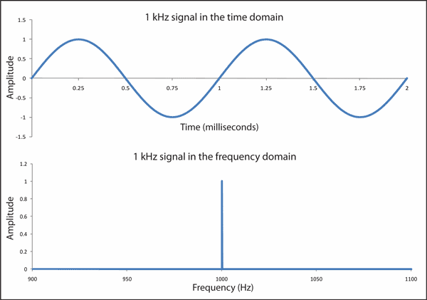
A pure sine wave has just one frequency, which in this case is 1kHz. So in the frequency domain plot, we see just one peak at 1kHz on the x-axis. Whatever frequency that the sine wave oscillates at determines where the peak will be in the frequency domain. This peak is mathematically known as an “impulse”. We can also see that the amplitude of the impulse in the frequency domain matches the amplitude of the sine wave.
What does this mean? Basically, we can apply the same idea of time domain signals being a sum of sinusoids to the frequency domain, where signals are a sum of impulses.
Going from time domain to frequency domain
To get the frequency domain representation of a signal, we need to transform the signal using what’s known as the Fourier Transform:
\[X(j\omega) = \int x(t) e^{j\omega t} dt\]We usually write the frequency domain representation of a signal using a capital letter. So $x(t)$ in time domain is $X(j\omega)$ in the frequency domain.
To go back to the time domain, we can do almost the same thing as the Fourier Transform, except we add a scaling factor. This is known as the Inverse Fourier Transform:
\[x(t) = \frac{1}{2\pi} \int X(j\omega) e^{j\omega t} d\omega\]Fourier Series Properties
Fourier series have a few properties that we can make use of to manipulate signals and understand what happens when we perform certain operations on them. It’s gonna be a lot to take in at once, so I’ll try to keep things as short as possible.
Linearity
Linearity is the most straightforward and can be summarized with the following expression:
\[ax(t) + by(t) \leftrightarrow aX(j\omega) + bY(j\omega)\]Basically, if you add two signals together in time domain, it is equivalent to adding the two signals in frequency domain. If you scale a signal by a constant scaling factor in time domain, it is also equivalent to scaling the signal in the frequency domain by the same scaling factor.
Time Shifting
The time shifting property states that if we shift a signal in the time domain by $t_0$, it is equivalent to shifting the phase of the signal by $-\omega t_0$ in the frequency domain.
\[x(t-t_0) \leftrightarrow e^{-j\omega t_0} X(j\omega)\]Conjugation
Conjugation states that if the frequency domain representation of $x(t)$ is $X(j\omega)$, then frequency domain representation of $x^{}(t)$ is $X^{}(-j\omega)$.
\[\text{If} \quad x(t) \leftrightarrow X(j\omega) \quad \text{then} \quad x^*(t) \leftrightarrow X(-j\omega)\]Frequency Shifting
If we shift a signal’s frequency by $\omega_0$, it is equivalent to multiplying the time domain signal by $e^{j\omega_0 t}$.
\[X(\omega - \omega_0) \leftrightarrow e^{j\omega_0 t}x(t)\]Duality
The Fourier Transform and Inverse Fourier Transform, while similar, are not exactly the same. This leads to a property that can be expressed as such:
\[X(t) \leftrightarrow 2\pi x(-\omega)\]If we form a new time domain function that has the functional form of the transform $X(t)$, it will have a Fourier Transform $x(\omega)$ that has the functional form of the original time domain function (except it is a function of frequency)
Convolution
The convolution property states that a convolution in time domain corresponds to a multiplication in the frequency domain. This means that we can use a Fourier Transform to avoid doing convolutions by converting them to multiplication.
\[x(t) * y(t) \leftrightarrow X(j\omega)Y(j\omega)\]Parseval’s Relation
Parseval’s relation states that the total energy of signal can be determined by computing the energy per unit time and integrating over all time or by computing the energy per unit frequency and integrating over all frequencies.
\[E = \int^{\infty}_{-\infty} |x(t)|^2 \ dt = \frac{1}{2\pi} \int^{\infty}_{-\infty} |X(j\omega)|^2 \ d\omega\]Phew, now that’s what you call an information overload. There are still more properties, but these are the more important ones to know (in my opinion). I won’t show how these properties are derived. If you’d like to the proofs for these properties, I’d recommend reading Signals and Systems by Oppenheim. If you can’t wrap your head around these equations, don’t worry. The important part is that we understand and use these properties to manipulate signals and see what happens when we process signals.