The Digital Domain

So far we’ve talked about signals with the understanding that they are continuous functions of time/frequency. However in the context of DSP, we can’t work with continuous signals. This is because continuous signals are an infinite and uncountable sequence of numbers, where each number itself also has an infinite number of possible values.

Because of this, computers can’t work with continuous signals, as that would require an storing an infinite amount of data. Therefore, we must first discretize a signal (make it finite and countable) before we can process it digitally.

If you’ve read my post about ADCs and DACs, we know that we can convert an analog (continuous) signal to a digital (discrete) signal using an ADC (analog-to-digital converter). ADCs perform this conversion by taking snapshots of the continuous signal at regular time intervals. This is known as sampling.

Sampling and Quantization

Digital signals approximate continuous signals via sampling. However, sampling has limits to the precision and range of the values that it can represent. This limitation is known as quantization.

Take for example a 4-bit ADC. If we try to sample a sine wave using a 4-bit ADC, we end up with the red curve.

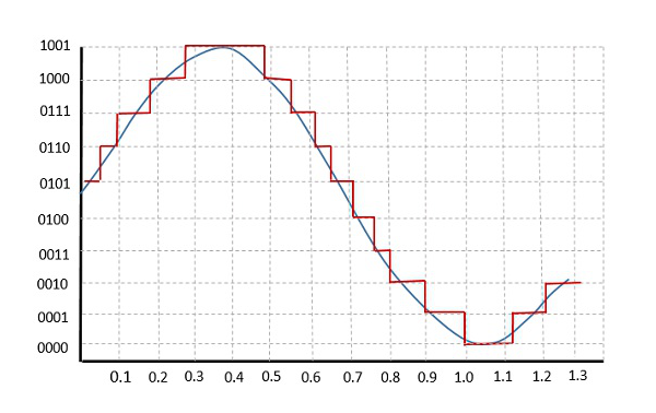
This happens because the resolution of the ADC is not high enough to accurately represent all of the values in the sine wave. As there is a limited number discrete values that we can use to represent signal values digitally, some signal values are forced to be rounded off so that it can be mapped to the nearest discrete value.

Hence, quantization imposes an upper limit to how accurate a continuous signal can be represented digitally. The more bits that we can use to represent the continuous signal, the higher the resolution and therefore the more accurately we can approximate the continuous signal.

Another thing that affects the accuracy of a discretized signal is the sampling rate which refers to how fast we sample a signal. The faster we sample, the more information we have about the signal, at the expense of storage space. Therefore, choosing an appropriate sampling rate for your application is important.

But we can’t just choose any sampling rate.

The Nyquist-Shannon Sampling Theorem

The Nyquist-Shannon Sampling Theorem (or just the Nyquist Theorem) states that if we want to be able to reconstruct a continuous signal from the discrete counterpart, it must be sampled at a rate that is at least twice the highest frequency that is present in the signal. This minimum sampling rate is known as the Nyquist rate.

The Nyquist frequency is a closely related term that tells you the maximum frequency component of a signal that can be accurately recorded given a certain sampling rate. For a given sampling rate, the Nyquist frequency is equal to half of the sampling rate.

So what’s with this seemingly arbitrary requirement? Well, sampling above the Nyquist rate helps avoid a phenomenon known as aliasing. Aliasing occurs when the high frequency components of a signal are mistaken for lower frequency components. This leads to distortion in the signal and makes it difficult for us to accurately reconstruct the continuous signal.

Luckily, aliasing is quite simple to deal with. We just need to run the signal through an anti-aliasing filter before sampling it. An anti-aliasing filter is essentially just a low-pass filter which removes all the frequency components that are higher than the maximum frequency we are interested in.

Take audio for example. The human hearing range is between 20Hz to 20kHz, so we can remove all of the frequency components in the audio that are above 20kHz so that we can avoid aliasing (and also because we can’t hear them anyway so why waste space storing them).

The Discrete Time Fourier Transform (DTFT)

If a continous-time signal is $x(t)$, then a discrete-time signal is $x[k]$, where $k$ is the sample. So $x[1]$ refers to the first sample of a continuous signal.

Therefore, we need to modify the Fourier Transform that we’ve discussed in the previous part such that it works with discrete-time signals. The expression is largely similar, with the difference being that the integral term is replaced with a summation and $x(t)$ is replaced with $x[k]$.

Hence the DTFT can be written as:

\[X(\omega) = \sum^{\infty}_{k = -\infty} x[k]e^{-j\omega k}\]

and the inverse DTFT is:

\[x[k] = \frac{1}{2\pi} \int_{0}^{2\pi} X(\omega) e^{j\omega k} \ d\omega\]

With the DTFT in our hands, we can now use it for DSP purposes, namely to obtain the frequency domain representations of discrete signals.

But there’s a catch. Computing the DTFT from the above definition is slow. Very much so. So instead, we use an alternative known as the Fast Fourier Transform or FFT for short. The FFT algorithm significantly reduces the time complexity of computing the DTFT from $O(n^2)$ to $O(n \log n)$. This is such a big deal that the FFT has been cited as the most important algorithm of our lifetime and was even included in a top 10 list of algorithms.

The FFT in Python

Alright, that’s enough theory for now. Let’s now look at some Python code to see how we can actually use the FFT and to see the FFT outputs of some signals. We’ll make use of Numpy’s built-in FFT function, np.fft.fft().

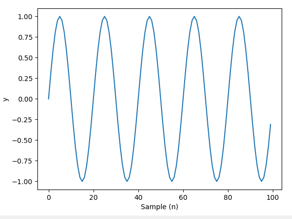
Let’s define a sine wave that oscillates with a frequency of 5Hz, along with the numer of samples that make up the signal and the sampling rate then take the FFT.

import numpy as np
import matplotlib.pyplot as plt

Fs = 8000
f = 5
sample = 8000
x = np.arange(sample)
y = np.sin(2 * np.pi * f * x / Fs)
plt.plot(x, y)
plt.xlabel('Sample (n)')
plt.ylabel('y')
plt.show()

The sine wave looks like this:

Taking the FFT:

Y = np.fft.fft(y)

The output will be an array of complex numbers. We can calculate the magnitude and phase of the complex numbers and plot them out.

Y_mag = np.abs(Y) 
Y_phase = np.angle(Y)

plt.subplot(1, 2, 1)
plt.plot(x, Y_mag, '.-')
plt.xlabel('Sample (n)')
plt.ylabel('Magnitude')

plt.subplot(1, 2, 2)
plt.plot(x, Y_phase, '.-')
plt.xlabel('Sample (n)')
plt.ylabel('Phase')
plt.show()

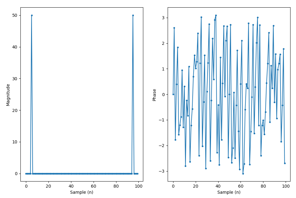
Right now, we’re just plotting out the FFT with the indices as the x-axis values, which doesn’t really make for a nice visualization. So we’ll need to do a few things.

By default, the FFT function returns the DFT results from 0Hz to the sampling frequency. But we’d like to visualize the FFT with the DC (0Hz) component in the middle of the spectrum so that we can see both the positive and negative frequency components in the FFT.

But hold on, what the heck is a negative frequency? To keep things simple, negative frequency is not a physical phenomenon but rather just a mathematical construct that we use in signal analysis and representation.

For real-valued signals, the FFT exhibits conjugation symmetry, meaning that the negative frequency components in the FFT mirrors the positive frequencies and thus are redundant.

So now we shift the FFT and plot it with 0Hz in the middle.

Y = np.fft.fftshift(np.fft.fft(y))
f = np.arange(-Fs/2, Fs/2, Fs/N)

plt.subplot(1, 2, 1)
plt.plot(f, Y_mag, '.-')
plt.xlabel('Frequency')
plt.ylabel('Magnitude')

plt.subplot(1, 2, 2)
plt.plot(f, Y_phase, '.-')
plt.xlabel('Frequency')
plt.ylabel('Phase')
plt.show()

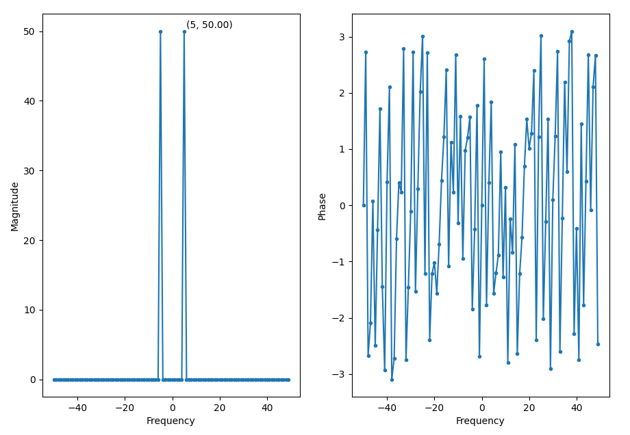
We can see a peak at 5Hz, which is the frequency of the sine wave.

Windowing

The FFT assumes that the input signal is periodic with a period $N$. So it analyzes the signal in chunks of $N$ samples. However, if the signal is not actually periodic (which is pretty common), then there’ll be discontinuities at the boundaries of the $N$ sample windows.

These discontinuities will appear as very high frequencies in the signal’s spectrum that are not present in the original signal. These frequencies can be higher than the Nyquist frequency and thus cause aliasing. This is known spectral leakage, as it appears as though the energy at one frequency has leaked into the other frequencies.

Thankfully, we can control this leakage via a technique known as windowing.

Windowing involves applying a window function to a signal that reduces the amplitude of the discontinuities at the boundaries of each $N$ sample block, making the signal taper off and gradually approach zero at the boundaries.

In general, all window function look something like this in the frequency domain:

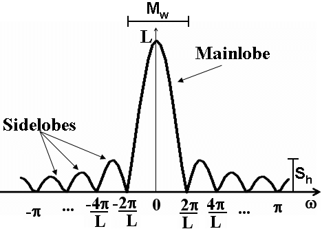
Selecting a window function is not a straightforward process, and largely depends on the characteristics of the signal you’re analyzing. Window functions have a few characteristics that we need to consider when selecting one:

The width of the main lobe
Side lobe height relative to the peak of the main lobe.
The roll-off rate of the side lobes (i.e. how fast they decay/die down)

The width of the main lobe determines the frequency resolution. A narrower main lobe gives better resolution, allowing us to distinugish closely spaced frequncies. However, a narrower main lobe also increases spectral leakage.

As for the side lobes, a lower side lobe height reduces spectral leakage, but makes the main lobe wider which lowers frequency resolution. A higher roll-off rate reduces spectral leakage.

Most of the time, a Hanning window works well enough for most scenarios. So if you’re not sure, you can always start with a Hanning window and see where it takes you.

FFT Size

The size of an FFT determines the frequency resolution of the transform. The larger the zsize, the larger the number of frequency bins. So a larger FFT gives you more details about a signal’s frequency spectrum. FFT sizes are always an order of 2 due to the way the algorithm works.

Spectrograms

A spectrogram is a plot of frequency over time. It’s basically a bunch of FFTs stacked on top of each other and typically looks something like this:

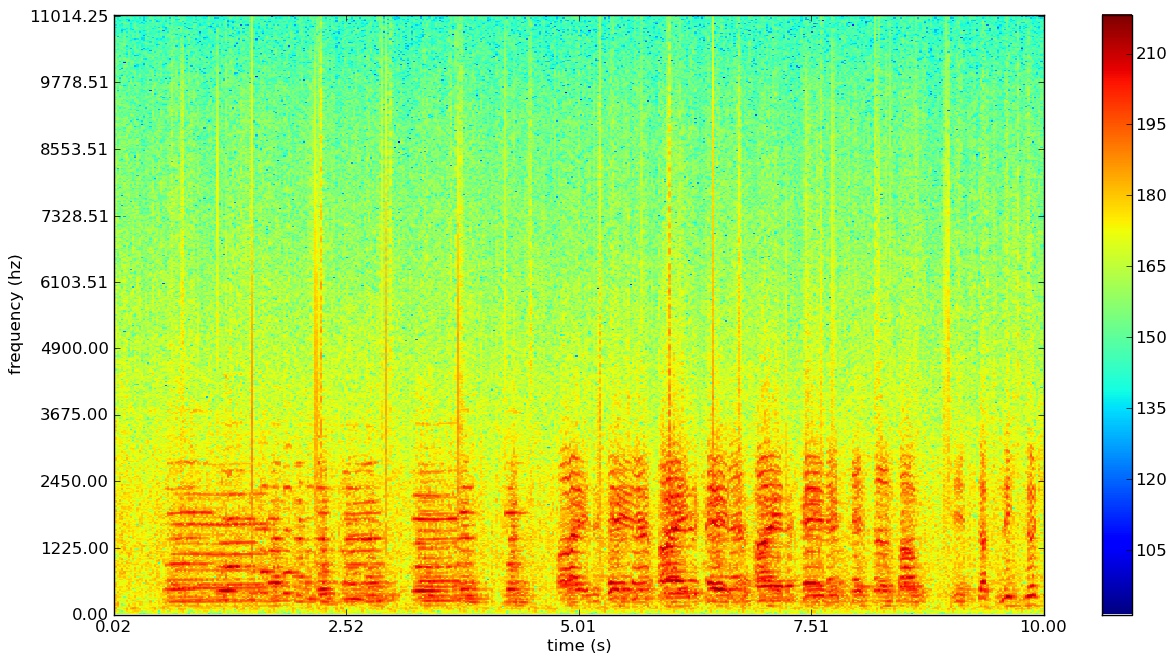
Based on the colourmap, we can use the red regions to identify at which points in time and at which frequencies that the energy of the signal is concentrated at.